Fig. 8.14 Inversion of the frequency axis: summary of the magnitude and phase Bode plots for the inverted real polo,

I GO-co) II,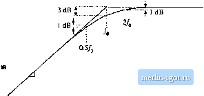

+20 dB/decade

+90°

/ Л0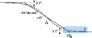

8.1,4 Frequency Inversion

Two other forms arise, from inversittn of the frequency axis. The inverted pole has the transfer function

(a.i-i)

As illustrated in Fig, S,14, the inverted pole has a high-frequency gain of 1, and a low frequency asymp-tt)te having a Ч-20 dB/decade slope. This form is useful for describing the guin of high-pass tillers, and of other transfer functions where it is desired to emphasize the high frequency gain, with attenuation of low-frequencies. Equatitm (8,35) is equivalent to

C(.!) =

(8.36)

However, Eq. (8.35) more directly emphasizes tliat the high frequency gain is 1. The inverted zero has the form

(8,37)

As illustrated in Fig. 8,15, the inverted zero has a high-frequency gain asymptote equal to 1, and a low-frequency asymptote having a slope equal to -20 dB/decade. An example of the use of this type of trans-

Converter Тпшфг Fuucfionx

II с(/ш) lu

-,-20 dB/deeade

Fig, S,1S Inversion ol llie frequency axis: summary of (he ningnimdc and phase Bode pior for Lhe inverted real zt№.

ZGiJw) -W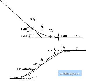

/ /10

fer function is the proportional-pius-integral controller, discussed in connection with feedback loop desigu in the next chapter Equation (8.37) is equivalent to

(ij.38)

However, Eq. (8.37) is the preferred form when it is desired to emphasize the value of the high-frequency gain asymptote.

The use of frequency inversion is illustrated by example in the next section. 8.1.5 Combinations

The Bode diagram of a transfer function contuining several pole, zero, and gain terms, can he constructed by simple additittn. At any given frequency, the magnitude (in decibels) of the cttmposite transfer function is equal to the sum of the decibel magnitudes of the individual terras. Likewise, at a given frequency the phase of the composite transfer function is equal to the sum of the phases of the individual terms.

For example, suppose thut we have already constructed the Bttde diugrums t)f twt) complex-valued functions of 0), G((j)) und G2((U), These functions have magnitudes Л(0)) and Rif), and phases ej(iu) and Й2(а)), respectively. It is desired to construct the Bode diagram of the prttdiict Cj(tu) = O((0)G2(Ci)). Let Оэ(Ш) have magnitude Л(Ш), and phase 6((li).To find this magnitude and phase, we can express ((ш), (O)), and f rj((J)) in polar form:

Cl{iii)R,Ыe

The product Gj(ti)) can then be expressed as

С,(ш) = С((0)(;з(ш) = /(.аде ! Й2(й))й-*2

Simplification leads tt)

Hence, the composite phine is Tiie total magnitude is

When exipressed in decibels, Eq. (8.43) becomes

(8.39)

(8.40)

(8.41)

(3.42)

(8.43)

(8.44)

So the composite phase is the sum tifthe individual phases, ami when expressed in decibels, the composite magnitude is the simi of the individual magnitudes. The composite magnitude slope, in dB per decade, is therefore also the sum ofthe individual .slopes in dB per decade.

II Gil

40dB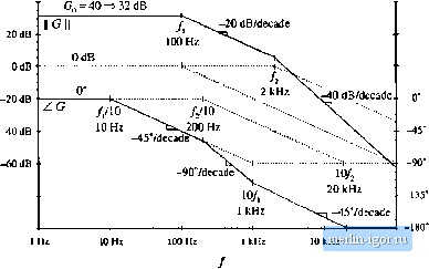

100 kHi

Fig. 8,16 Conatruclion of magnitude and phase asymptotes for the ttansler function of Eq,(B.45). Dashed line