I4.i Miiltiple-Windiii Manelics Design via itie KMelkod 547

The low-frequency copper loss P in winding 7 depends on the dc resistance Л. of winding j, as follows:

P..ii]Pt (i -)

The resistance of winding / is

(14,25)

Avij

where p is the wire resistivity, £y is the length of the wire used for winding/, and Ащ is the ctoss-sectionai area ofthe wire used for winding /. These quantities can he expressed as

ljHj(MLT) (14.26)

A.j = 4f (14,27)

where {MLT) is the winding raean-length-per-turn, and /f, is the winding fill factor. Suhstitution of these expressions into Eq. (14.25) leads to

The copper loss of winding / is therefore

The total copper loss ofthe к windings i.s

(14.30)

It is desired to choose the such that the total copper loss P j, is minimized. Let us consider what happens when we vary one of the as, say (Xj, between 0and 1.

When a, =0, then we allocate zero area to winding 1. In consequence, the resistance of winding 1 tends to infinity. The topper loss of winding 1 also tends to infinity. On the other hand, the other windings are given maximum area, and hence their copper losses can be reduced. Nonetheless, the total copper loss tends to infinity.

When a, = l,then we allocate all ofthe window area to winding 1, and none to the other windings. Hence, the resistance of winding 1, as well as its low-frequency copper loss, are minimized. But the copper losses ofthe remaining windings tend to infinity.

As illustrated in Fig. 14.8, there must be an optimum value of [ that lies between these two extremes, where the total copper loss is minimized. Let us cotnpute the optimum values of Ci, ctj,ftj using the method of Lagrange tnultipliers. It is desired to tninitnize Eq. (14.30), subject to the cotistraint of Eq. (14.23). Hence, we define the function

Copper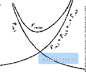

Fig. 14.S Variation of copper losses with a[.

1 a,

04.3!)

where

(14,32)

is the constraint that must etjiiai zero, and is the Lagrange multiplier. The optimum point is the solution of the system of equations

tfotj

3/(a aj,--,a )

dec.

a/(a,.(j;.--.r(.,)

(14.33)

The solution is

p(Mi,T)f.

(14.34)

(14.35)

This is the optimal choice for the as, and theresulting minimum valueof P .

According to Eq. (14,22), the winding voltages are proportional to the turns ratios. Hence, we can expiess the a-S in the alternate form

(14.36)

by multiplying and dividing Eq. (14.35) by tlie quantity V /fi ,. It i.4 irrelevant whether rms or peak volt-age.4 are used. Equation (14.36) is the desired result. Il .states that the window area should be allocated to the various windings in proportion lo their apparent powers. The numerator of Eq. (14.36) is the apparent power of winding m, equal lo the product of the rms current and the voltage. The denominator is the sum of the apparent powers of all windings.

As an exaraple. consider the PWM full-bridge transforraer having a center-tapped secondaty. as illustrated in Fig. 14.9. This can be viewed as a three-win ding transformer, having a single primary-side winding of turns, and two secondary-side windings, each of n, turns. The winding current waveforms !j(f), iit), and 1з(() are iilnstrated in Fig. 14.10. Tlieir rms values are

(14.37)

(14,38)

Substitution of these expressions into Eq. (14.35) yields

- I

.tt7t V £}-

(14.39)

(14.40)

If the design is to be optimized at the operating point D - 0.15, then one obtains

a, = 0396 2 = 0,302 a, = 0,302

(14.41)

So appToxiraateiy 40% of the window area should be allocated to the priraary winding, and 30% should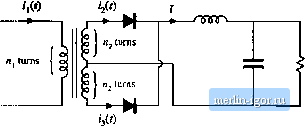

Fig, 14,9 PWM full-bridge transformer example.